Spreadsheet Basics

Download PDF version (289.5k) Log In or Register to view the full article as a PDF document.

If I had to choose just one piece of software with which to run my business, it would be the spreadsheet. This is as true today, when I work on a state-of-the-art Pentium machine, as it was when I purchased my first IBM XT clone more than 15 years ago. Over the years, I’ve used spreadsheets for the usual purposes — estimating, invoicing, and job-costing — and the unusual — figuring cuts for rake walls or hip roofs. I have even heard of a contractor who used a spreadsheet to lay out a tile pattern for a shower. Most new computers come with software, such as Microsoft Works or Claris Works, that includes a spreadsheet. If you spend a few hours learning how to use a spreadsheet, you’ll begin to find ways to put it to work in your business, without having to spend another cent on software. In this article, I’ll use a couple of simple spreadsheets I set up when I first started using a computer to explain how spreadsheets work. But those are just the tip of the iceberg. Once you feel comfortable with these simple examples, you’ll find that’s it’s easy to set up more complex spreadsheets to fit your business.

Rows and Columns

If you have ever used a columnar pad to estimate or do your bookkeeping, then perhaps without realizing it, you’ve used a manual version of a spreadsheet. Spreadsheet software builds on the row-and-column structure of a paper columnar pad, adding automated shortcuts and other features that make the job of entering and manipulating data easier. The biggest advantage a spreadsheet has over a paper columnar pad is that a spreadsheet will do all the math for you. Even if you use a calculator to estimate, it’s tedious to add up all your labor, material, and subcontractor costs across each row, then total the columns. If you’re interrupted midstream, it’s easy to forget where you left off. And changes — like a call from the architect telling you to use $6 per square foot for tile instead of $5 — mean you have to start all over again. After all that, your client may still get this strange smile on his face during your presentation, causing you to wonder if your price is $20,000 too low because you made some math error. A spreadsheet takes the guesswork and the tedium out of all of these situations. A spreadsheet can link individual entries, or "cells," in the rows and columns so that when the value of one cell changes, the values in all linked cells change, too. The process is accurate and it all happens in the blink of an eye.

Estimating

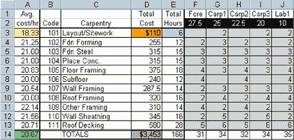
When I first started using a computer in my business, I did almost everything on a spreadsheet. Early on, the most pressing issue was to be able to estimate and feel confident that I had not made any math errors. At the time, I was using my best judgment as to how long each component would take to build, since almost everything we did was custom and I had not yet done enough job-costing to come up with square-foot or linear-foot costs for labor. So I set up a "template" with a list of labor items I used regularly to estimate labor for the job (see Figure 1).

=SUM(F3:J3)

=(F3Foreman)+(G3Carpenter1)+(H3Carpenter2)+(I3Carpenter3)+(J3Laborer1)*

=SUM(D3:D13)

=IF(E3=0,"0",D3/E3

=AVERAGE(A3:A13)

Figure 1. The rows in this labor-estimating template correspond to specific tasks, which are coded and listed in columns B and C. Hours for each employee are entered in columns F through J. The formulas that fill columns A, D, and E (colored cells) calculate totals. I used the template as a worksheet to do my estimating and to track my labor costs once the job was underway. The layout of this template is simple. Columns B and C hold task codes and descriptions, and match those on my company’s timesheets. Each of the columns F through J correspond to one of my employees, and the headings of these columns (cells F1 through J1) hold job descriptions, such as "Foreman," "Laborer," or one of several skill levels of "Carpenter." Immediately below (cells F2 through J2) is the hourly wage for each job description. The cells in the other three columns (A, D, & E) hold formulas that perform math calculations on the numbers I enter in each row; the cells in row 14 hold formulas that total the columns.

Adding numbers in rows.

When I do a labor estimate, I follow the list of tasks, row by row, entering the number of hours I think each employee will spend on each one into the cells under each job description (columns F through J). To find the total hours estimated for a given task, column E (labeled "Total Hours") holds a formula that adds the hours, row by row, from the job description columns. In cell E3, for example, the formula looks like this: =SUM(F3:J3)
If you key this formula in directly, you have to be careful to include the correct symbols in the proper position. You can save time and reduce the chances of making a typo by using one of two other ways to enter the formula. One method is to click on the function button, which calls up a list of available functions (Figure 2).

Figure 2. The easiest way to enter a formula is to pick from a list, such as this one in Excel (top). Clicking on the SUM function, for example, opens a dialogue box (bottom), which walks you through the formula. After choosing SUM from the list, a dialogue box opens and walks you through the formula. During this process, you can use the keyboard or mouse to select the cells you want to add. Because the SUM function is used so often in most spreadsheets, there’s a second, easier way to enter the formula: Just click on the SUM button on the toolbar at the top of the screen. This button takes you directly to the dialogue box for the SUM function.

Adding numbers in columns.

The SUM function works with columns of numbers, too. In my labor estimating template, for example, the formula in cell D14 looks like this: =SUM(D3:D13)
Like the other formulas in row 14, this formula adds together all of the values in the column above it. Absolute references.
So far, we’ve looked at formulas that operate on cells based on their position relative to each other. For example, the SUM formula in cell E3 operates on the five cells immediately to the right (F3:J3). If we were to copy this formula into the cell just below (E4), the spreadsheet would automatically change the references from F3:J3 to F4:J4, because these cells are immediately to the right of E4. Sometimes, however, I need to use an "absolute reference" — a formula that operates on the same cell no matter where on the spreadsheet the formula is located. The formulas in column D of my template use absolute references to calculate the labor costs for each employee and add them together to get the total cost of each task. In cell D3, for instance, the formula first multiplies the number of hours in cell F3 times the hourly rate in cell F2; it does the same for each of the other four cells in the row and adds them all together. One cell down in D4, however, the formula again refers to cell F2, even though cell F2 is not located in the row directly above. If this formula used relative references, it would look like this: =(F3*F2)+(G3*G2)+(H3*H2)+(I3*I2)+(J3*J2)
Using absolute references, it looks like this: =(F3*$F$2)+(G3*$G$2)+(H3*$H$2)+(I3*$I$2)+(J3*$J$2)
The dollar signs indicate that the formula should reference this cell no matter where the formula is located on the spreadsheet. Naming cells.
You have to be careful when copying formulas that use absolute references from one cell to another. Most spreadsheets assume that all references are relative, so you have to manually go into each copied formula and add the dollar signs. An easy way to work around this problem is to give the absolute reference cells a name. In my template, for example, the cells that hold wage amounts are named "Foreman," "Carpenter 1," Carpenter 2," and so on. Using these names, the formula in cell D3 looks like this: