In my past job as an estimator for a lumberyard, I did hundreds of material takeoffs every year, and I still do them in my current job as an architectural draftsman. Some estimators use specialized software, but I estimate the same way many contractors do — with a spreadsheet. Almost any spreadsheet will do; I happen to use Excel.
You can create a spreadsheet estimating template without knowing more than a few basic functions — how to add, subtract, multiply, and divide. But it’s worth taking the time to learn a few more advanced functions: Not only will you be able to use them in your estimating spreadsheet, but you’ll be able to create spreadsheets for many other construction calculations as well.
Estimating materials is all about calculating areas and volumes — something you can do faster and more reliably with a spreadsheet than with a calculator. When you use a template, the formulas are already in place, so all you have to do is key in dimensions from the prints, which greatly reduces the chance for keystroke errors.
My estimating template has many worksheets, or tabs. Since the worksheets for the roof contain many advanced functions, I’ll use them to show how the template works. Most of the buildings I estimate use trusses, so the template isn’t set up to estimate rafters. It does, however, contain worksheets for other roof components, like sheathing, finish roofing material, and wood and metal trim.
Roof Area Calculations
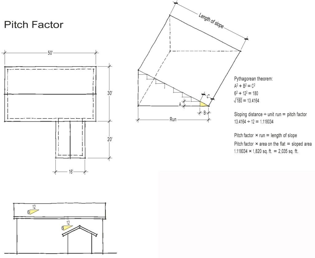
The first thing I do when estimating a roof is figure out its area. For the purpose of this article, let’s say we’re looking at a simple L-shaped house with a pair of 6/12 gables. The plans indicate that, including overhangs, the roof measures 1,820 square feet on the flat. But since the sloping area is greater than the flat area, you’ll need more material than that.
You could scale the slope distance from an elevation and use it to calculate the area of the roof, but as an estimator I’ve learned not to scale from prints. It’s too easy to make a mistake, especially when they’re drawn to 1/4-inch or 1/8-inch scale. Plus, if the prints were drawn by hand or subsequently copied, they may not actually be to scale.
Pitch factor. I prefer to put a formula in the template and let the spreadsheet calculate the slope. It’s faster than using a calculator and there’s less chance of a mistake. All I have to do is enter the area on the flat in one cell and the pitch in another, and the template creates a pitch factor, which it uses to calculate the sloped area of the roof (see Figure 1).
The pitch factor is the ratio between the sloping distance and the run. Multiplying the area on the flat by this number gives you the area on the slope. To calculate a pitch factor, start with the Pythagorean theorem:
A2 + B2 = C2
A is the rise, B is the run, and C is the sloping distance. For a 6/12 roof, A equals 6, B equals 12, and C equals the square root of 180 (62 + 122). The square root of 180 is 13.4164. The formula for the pitch factor is:
sloping distance / unit run = pitch factor
13.4164 / 12 = 1.118034
Think of this number as a percentage: Rounded up, it tells us that the distance up the slope of a 6/12 roof is 112 percent of the horizontal run.
With the pitch factor, we can easily determine the sloped area of the roof:
pitch factor x area on the flat = sloped area of the roof
1.118034 x 1,820 sq. ft. = 2,035 sq. ft.
This formula will work for any roof where all the areas are the same pitch. If the roof has more than one pitch, then you’ll have to use separate pitch factors for each area. The estimating template has been simplified for this story; my regular estimating template contains additional rows that can be used when the roof has more than one pitch.
Putting the Formula Into Excel
While a carpenter may understand these formulas, Excel can’t use them unless they’re written in a certain format. Squaring a number, as in 62, is the same as raising the number to the second power.
In Excel, you can square the number 6 by entering this formula into a cell:
=POWER(6,2)
That tells the program to raise the number 6 to the power of 2. To square the number 4 you’d enter =POWER(4,2). If you wanted to cube the number 6 (raise it to the third power), you would enter =POWER(6,3).
We need to convert A2 + B2 = C2 into language that Excel can understand. Since we’re talking about a 6/12 roof, the calculation would be:
(6)2 + (12)2 = C2
As you’ve guessed, the convention for entering a formula in Excel is to put an equal sign in front of it. So for a 6/12 roof the cell entry to solve for C2 would be:
=POWER(6,2)+POWER(12,2)
Since we usually work in pitches that show a rise over 12, we can simplify the formula by using the number 144 (12 squared) in place of the second POWER function. The simplified entry would be:
=POWER(6,2)+144
Some plans show rise over 10. In that case you would substitute the number 100 (102) for 144.
Finding the Square Root
To find the sloping distance of a 6/12 roof, we must solve for C in the equation A2 + B2 = C2. So far, we’ve only entered A2 + B2. C is the square root of A2 + B2. To find the square root, we add =SQRT in front of the formula:
=SQRT(POWER(6,2)+144)
Note the outer set of parentheses, which tells Excel to treat (Power(6,2)+144) as a single number. (There should always be the same number of parentheses facing left as there are facing right.)
The result is 13.41641. To convert this number to a pitch factor, you divide it by 12. The formula will now read:
=SQRT(POWER(6,2)+144)/12
The result is 1.118034 — the pitch factor. To find the sloped roof area of the roof described above, we can now multiply by the area on the flat (1,820 square feet). The formula now reads:
=1820*SQRT(POWER(6,2)+144)/12
The result is 2,035, the square footage of sheathing needed for the roof.
This formula is not quite ready to be put into the estimating template. The way it reads now, you would have to change some of the numbers every time you did an estimate. For example, if the roof had a 7/12 pitch, you’d have to change the 6 to a 7. And if the roof was 2,500 sq. ft. on the flat, you’d have to change 1,820 sq. ft. to 2,500 sq. ft.
It would be much better to put the formula into the template once and then leave it alone. The way to do that is to use cell references for the values that change.
Cell References
A cell reference tells Excel where to find a particular piece of data. This saves you from having to enter the same number multiple times and places — an incredibly useful function that’s worth mastering.
So instead of changing the roof area formula for every estimate, I substitute cell references for the values that change (Figure 2). On the miscellaneous roof framing tab, the area on the flat (1,820) is in cell E8 and the pitch (6) is in E9. With these cell references, the formula reads:
=E8*SQRT(POWER(E9,2)+144)/12
With this formula in place, we can enter any area on the flat we want in E8 and any pitch we want in E9 and the spreadsheet will automatically calculate the sloped area of that roof.
Creating references between tabs. In the formula above, the cell references apply to cells on the same worksheet. But what if you want to refer to cells on a different worksheet?
For example, the area of roof that has to be sheathed was calculated on the miscellaneous roof framing tab, but I need to use the same number to estimate shingles on the tab for roof covering. I could manually transfer this number to the roof covering tab, but it would be safer and faster to do it by creating a reference to a cell on a different tab. That way, if a design change alters the amount of roof sheathing, the shingle quantity automatically updates to the correct amount.
Rounding Up to Full Pieces
If you wanted to sheathe an 8-foot-by-10-foot area, you’d need 80 square feet of plywood or OSB. That’s two-and-a-half sheets, but since you can’t buy half sheets you’ll have to round up to three sheets to sheathe that area. You can tell the spreadsheet to do this by using the ROUNDUP function.
Be aware that this is different from formatting a cell to simply round to the nearest full number, because the cell could just as easily round down.
The ROUNDUP function can be found in many places within my estimating template. For example, on tab 29-CSF the spreadsheet calculates the number of 16-foot pieces of 1×8 cedar it will take to trim the rakes and eaves. The formula, in cell 11G, reads:
=ROUNDUP(I2*(1+I11)/16,0)
Note that the formula is telling the spreadsheet to take the value from I2 (210 lineal feet of fascia) and multiply it by 1 plus the value in cell I11 (a 10 percent waste factor).
I2*(1+I11)
210 x (1 + .1)
210 x 1.1 = 231
We want to buy 16-foot pieces of stock, so we divide the 231 lineal feet of trim by 16. The formula now reads:
I2*(1+I11)/16
231/16 = 14.44
We can’t buy 14.44 pieces of trim, which is why I’ve used the ROUNDUP function. Note the comma followed by 0 after the 16, which tells Excel to go to the next full number, which is 15. If you were to replace that 0 with a 1, it would round up to the nearest tenth, and the result would be 14.5.
Using the IF Function
Occasionally I’ll have to make a choice between two or more types of materials. For example, does the job call for 15-pound or 30-pound felt? In a case like this, you can use the IF function to quickly specify quantities.
Because you’re working from a template, you’ll have a line for every type of material you might use on a job, even though you won’t necessarily use every material on every job. There will also be a separate formula to calculate the quantity of each material. So you need a way to tell the spreadsheet which calculations to perform.
For instance, if you’re estimating 15-pound felt, you don’t want the spreadsheet to also calculate the quantity of 30-pound felt — you want one or the other.
I use the IF function in this situation. Cell E9 of sheet 27-RC allows me to specify which weight of felt to estimate. Entering a 1 means 30-pound felt; leaving a zero indicates 15-pound. Below, in G15, the formula reads:
=ROUNDUP(IF(E9=0,(E3/432)*(1+I15)),0)
This tells Excel, if E9 is a zero, to calculate the rolls of 15-pound felt by dividing the area of the roof to be shingled (2,035 square feet, in cell E3) by the number of square feet in a roll (432), multiplying by a waste factor (here, 0), then rounding up. If I had typed a 1 in E9, the worksheet would have calculated rolls of 30-pound felt, using the formula in G16:
=ROUNDUP(IF(E9=1,(E3/216)*(1+I16)),0)
Protecting Cells
To avoid accidentally changing a formula in the template, I “lock” the cells that remain the same for every estimate. That way, an errant keystroke won’t mess up the template and affect calculations.
The cells in the worksheet are color-coded. I use the yellow cells to enter the lengths and areas I take off the prints; these are the only cells that are intended to change. The unshaded cells in the column labeled “Qty” contain formulas that refer to the numbers in yellow. The numerical values in the white cells may change but the underlying formulas do not. Using the template is simply a matter of entering numbers in the yellow cells and letting the white cells perform calculations.
Bill Lacey is a former lumberyard estimator and the co-owner of Visual Dynamics, LLC, an architectural drafting and design company in Racine, Wis.
Download for Easier Reading
As you read this article, you can open the author’s estimating spreadsheet and follow along. To download the spreadsheet, go to www.jlconline.com/spreadsheets